Set up
library (akldogs)library (tidyverse)
── Attaching core tidyverse packages ──────────────────────── tidyverse 2.0.0 ──
✔ dplyr     1.2.0     ✔ readr     2.1.6
✔ forcats   1.0.1     ✔ stringr   1.6.0
✔ ggplot2   4.0.2     ✔ tibble    3.3.1
✔ lubridate 1.9.5     ✔ tidyr     1.3.2
✔ purrr     1.2.1
── Conflicts ────────────────────────────────────────── tidyverse_conflicts() ──
✖ dplyr::filter() masks stats::filter()
✖ dplyr::lag()    masks stats::lag()
ℹ Use the conflicted package (<http://conflicted.r-lib.org/>) to force all conflicts to become errors
library (tidytext)library (fs)library (knitr)library (kableExtra)
Attaching package: 'kableExtra'

The following object is masked from 'package:dplyr':

    group_rows
library (patchwork)library (scales)
Attaching package: 'scales'

The following object is masked from 'package:purrr':

    discard

The following object is masked from 'package:readr':

    col_factor
Attaching package: 'Hmisc'

The following objects are masked from 'package:dplyr':

    src, summarize

The following objects are masked from 'package:base':

    format.pval, units
Attaching package: 'plotly'

The following object is masked from 'package:Hmisc':

    subplot

The following object is masked from 'package:ggplot2':

    last_plot

The following object is masked from 'package:stats':

    filter

The following object is masked from 'package:graphics':

    layout
source ("../R/functions.R" )source ("../R/theme.R" )
<- list.files ("../data" , pattern = "am-reports" , full.names = TRUE )<- report_files |> path_file () |> path_ext_remove () |> str_extract ("[^-]+$" )<- report_files |> set_names (report_names) |> map (read_csv)
Rows: 96 Columns: 3
── Column specification ────────────────────────────────────────────────────────
Delimiter: ","
chr (1): category
dbl (2): year, count

ℹ Use `spec()` to retrieve the full column specification for this data.
ℹ Specify the column types or set `show_col_types = FALSE` to quiet this message.
Rows: 48 Columns: 3
── Column specification ────────────────────────────────────────────────────────
Delimiter: ","
chr (1): category
dbl (2): year, count

ℹ Use `spec()` to retrieve the full column specification for this data.
ℹ Specify the column types or set `show_col_types = FALSE` to quiet this message.
Rows: 108 Columns: 3
── Column specification ────────────────────────────────────────────────────────
Delimiter: ","
chr (1): category
dbl (2): year, count

ℹ Use `spec()` to retrieve the full column specification for this data.
ℹ Specify the column types or set `show_col_types = FALSE` to quiet this message.
Rows: 224 Columns: 3
── Column specification ────────────────────────────────────────────────────────
Delimiter: ","
chr (1): category
dbl (2): year, count

ℹ Use `spec()` to retrieve the full column specification for this data.
ℹ Specify the column types or set `show_col_types = FALSE` to quiet this message.
Simplify some column names
<- registration |> rename (suburb = suburb_name)<- rename (rfs, suburb = location_suburb_name)
Auckland Dog Population Overview
As the dog population has increased, rates of registration and desexing have fallen, while rates of menacing dog ownership have increased.
<- $ ownership |> pivot_wider (names_from = category,values_from = count|> arrange (year) |> mutate (prev_value = lag (dogs),change = dogs - prev_value,pc_change = change / dogs,reg_pc = registered / dogs,desex_pc = desexed / dogs,men_pc = menacing / dogs|> select (year, dogs, pc_change: men_pc) |> arrange (desc (year)) |> rename ("Year" = year,"Known Dogs" = dogs,"Pop. Change" = pc_change,"Registered" = reg_pc,"Desexed" = desex_pc,"Menacing" = men_pc|> mutate (across ("Pop. Change" : "Menacing" ,~ scales:: percent (., accuracy = 0.1 )),"Known Dogs" = format (` Known Dogs ` , big.mark = "," )|> kable () |> kable_styling (full_width = FALSE ) Standarise the spelling of primary breeds
<- akldogs:: breeds<- registration |> left_join (breed_lookup, by = c ("animal_breed_description" = "raw_name" )) |> rename (breed_standardised = standardised_name) |> relocate (breed_standardised, .after = animal_breed_description)<- impounds |> left_join (breed_lookup, by = c ("primary_breed" = "raw_name" )) |> rename (breed_standardised = standardised_name) |> relocate (breed_standardised, .after = primary_breed) Investigate breed mismatches between registration and impound data.
The breed recorded in impound data does not match the breed for the dog with the same animal_id in the registration data, in over 6,000 cases. The rest of the analyses in this notebook use the data as provided by Animal Management, but noting this for follow up.
# Unique animals in impound data <- impounds |> select (dog_id) |> unique ()nrow (impounds_unique)
<- inner_join (|> select (animal_id, breed_reg = clean_name),|> select (dog_id, breed_imp = clean_name),by = c ("animal_id" = "dog_id" )|> unique () |> mutate (is_match = (breed_reg == breed_imp))
Warning in inner_join(select(registration, animal_id, breed_reg = clean_name), : Detected an unexpected many-to-many relationship between `x` and `y`.
ℹ Row 13 of `x` matches multiple rows in `y`.
ℹ Row 198 of `y` matches multiple rows in `x`.
ℹ If a many-to-many relationship is expected, set `relationship =
  "many-to-many"` to silence this warning.
<- comparison_by_id |> summarise (total_dogs_checked = n (),perfect_matches = sum (is_match),mismatches = sum (! is_match),accuracy_rate = mean (is_match) * 100 64.8% of unique dogs in the impound data, identified by their animal id number, have a different breed listed in the registration data. In many cases, this appears to reflect thedifficulty in identifying breeds visually, hence why many pit bull type breeds are grouped under ‘Pit Bull Terrier’.
But there are also many cases of dogs which appear visually distinct having mismatched breeds between the impound and registration data.
<- comparison_by_id |> filter (! is_match) |> count (breed_reg, breed_imp, sort = TRUE ) |> rename (reg_says = breed_reg,impound_says = breed_imp,frequency = nhead (top_mismatches, n = 10 )
# A tibble: 10 × 3
   reg_says                       impound_says                   frequency
   <chr>                          <chr>                              <int>
 1 American Pit Bull Terrier      Pit Bull Terrier                     886
 2 Fox (Smooth) Terrier           Fox Terrier (Smooth)                  64
 3 Staffordshire Bull Terrier     Pit Bull Terrier                      61
 4 American Staffordshire Terrier Pit Bull Terrier                      36
 5 American Staffordshire Terrier Staffordshire Bull Terrier            33
 6 Staffordshire Bull Terrier     American Staffordshire Terrier        32
 7 Labrador Retriever             Pit Bull Terrier                      30
 8 Labrador Retriever             Staffordshire Bull Terrier            28
 9 American Pit Bull Terrier      Staffordshire Bull Terrier            27
10 Labrador Retriever             Mastiff                               25
Top 10 primary breeds as at FY2025:
<- registration |> filter (sheet_name == "FY25" ) |> calc_proportions ("breed_standardised" , count_name = "primary_breed" )|> rename ("Breed" = breed_standardised,"Count" = primary_breed,"Proportion" = prop|> mutate (Proportion = scales:: percent (Proportion, accuracy = 0.1 ),Count = format (Count, big.mark = "," )|> head (n = 10 ) |> kable () |> kable_styling () Dog population secondary breed counts
<- registration |> filter (sheet_name == "FY25" ) |> calc_proportions ("animal_breed2_description" , count_name = "secondary_breed" )head (secondary_breed, n = 10 )
# A tibble: 10 × 3
   animal_breed2_description      secondary_breed   prop
   <chr>                                    <int>  <dbl>
 1 <NA>                                     75366 0.575
 2 Cross                                    19253 0.147
 3 Poodle, Miniature                         3190 0.0243
 4 Poodle, Standard                          2885 0.0220
 5 Retriever, Labrador                       2861 0.0218
 6 Poodle, Toy                               1802 0.0137
 7 Terrier, Staffordshire Bull               1789 0.0136
 8 Spaniel, Cavalier King Charles            1519 0.0116
 9 Shih Tzu                                  1501 0.0114
10 Collie, Border                            1393 0.0106
Primary breeds most commonly classified as ‘menacing’ due to behaviour
<- |> filter (sheet_name == "FY25" ) |> filter (classification == "Menacing - observed or reported behaviour of dog" ) |> count (breed_standardised, name = "menacing" ) |> left_join (primary_breed |> rename (primary_prop = prop), by = join_by (breed_standardised)) |> filter (primary_breed > 100 ) |> mutate (menacing_prop = menacing / primary_breed) |> arrange (desc (menacing_prop)) head (menacing_breed, n = 10 )
# A tibble: 10 × 5
   breed_standardised menacing primary_breed primary_prop menacing_prop
   <chr>                 <int>         <int>        <dbl>         <dbl>
 1 Akita                     8           102     0.000778        0.0784
 2 Siberian Husky           63          1330     0.0101          0.0474
 3 American Bulldog         66          1707     0.0130          0.0387
 4 Neapolitan Mastiff       11           293     0.00223         0.0375
 5 Mastiff                  57          1526     0.0116          0.0374
 6 Shar Pei                 71          2445     0.0186          0.0290
 7 Dogue de Bordeaux         4           139     0.00106         0.0288
 8 Weimaraner                4           152     0.00116         0.0263
 9 Bull Terrier             16           666     0.00508         0.0240
10 Bull Mastiff             24          1077     0.00821         0.0223
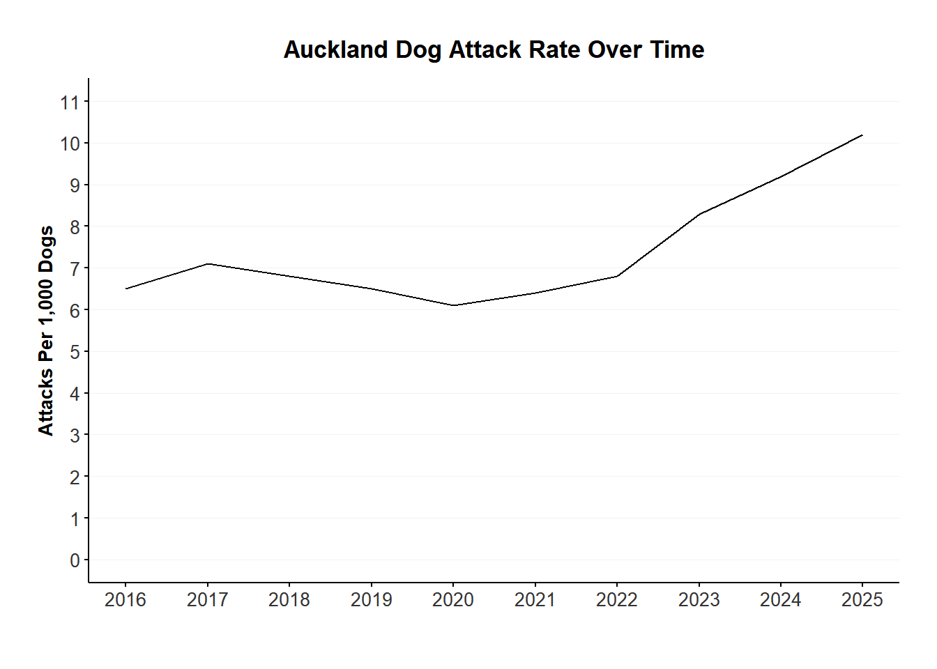
The rate of attacks on people per 1,000 dogs has increased from 6 in FY2016, to 10 in FY2025.
<- $ service |> filter (category == "attack-people" ) |> select (- category) |> rename (count_attacks = count) |> left_join ($ ownership |> filter (category == "dogs" ) |> select (- category) |> rename (count_dogs = count),by = join_by (year)) |> mutate (attack_rate = round ((count_attacks / count_dogs) * 1000 , digits = 1 ),head (attack_rate, n = 10 )
# A tibble: 10 × 4
    year count_attacks count_dogs attack_rate
   <dbl>         <dbl>      <dbl>       <dbl>
 1  2025          1341     131123        10.2
 2  2024          1253     135546         9.2
 3  2023          1098     131795         8.3
 4  2022           848     125016         6.8
 5  2021           756     118552         6.4
 6  2020           685     112530         6.1
 7  2019           716     110969         6.5
 8  2018           745     110012         6.8
 9  2017           816     115544         7.1
10  2016           740     114519         6.5
ggplot (attack_rate |> filter (year > 2015 ), aes (x = year, y = attack_rate)) + geom_line () + scale_y_continuous (limits = c (0 , 11 ), breaks = seq (0 , 11 , by = 1 )) + scale_x_continuous (breaks = 2016 : max (attack_rate$ year)) + xlab ("" ) + ylab ("Attacks Per 1,000 Dogs" ) + plot_theme () + labs (title = "Auckland Dog Attack Rate Over Time" ) Impounds
<- $ ownership |> filter (category == "dogs" ) |> rename ("dogs" = "count" ) |> select (- category) |> left_join (report_data$ impounds |> filter (category == "impounds" ),by = join_by (year)) |> rename ("impounds" = "count" ) |> select (- category) |> mutate (impound_rate = round ((impounds / dogs) * 1000 , digits = 1 )|> rename ("Year" = year,"Known Dogs" = dogs,"Impounded Dogs" = impounds,"Impound Rate" = impound_rate|> mutate (across (c (` Known Dogs ` , ` Impounded Dogs ` ), ~ format (.,big.mark = "," ))|> kable () |> kable_styling () Look at repeat impounds
<- impounds |> drop_na (dog_id) |> group_by (dog_id) |> add_count (name = "impounded_n" ) |> ungroup () |> select (dog_id, impounded_n, impound_date, impound_reason, status, suburb, desexed, clean_name) |> group_by (dog_id) |> reframe (impounded_n = impounded_n,reason = impound_reason,breed = clean_name|> arrange (desc (impounded_n)) |> select (dog_id, impounded_n, breed) |> unique ()|> count (impounded_n) |> mutate (proportion = n / sum (n))
# A tibble: 13 × 3
   impounded_n     n proportion
         <int> <int>      <dbl>
 1           1  5452   0.755
 2           2  1122   0.155
 3           3   352   0.0487
 4           4   155   0.0215
 5           5    50   0.00692
 6           6    33   0.00457
 7           7    20   0.00277
 8           8    24   0.00332
 9           9     3   0.000415
10          10     5   0.000692
11          12     2   0.000277
12          18     2   0.000277
13          20     1   0.000138
Top 3 primary breeds for each attack severity rating for impounded dogs in FY2024
<- |> filter (impound_date > "2023-07-01" & ! is.na (severity)) |> group_by (severity) |> count (breed_standardised) |> arrange (desc (severity), desc (n))|> group_by (severity) |> slice_max (order_by = n, n = 3 ) |> arrange (desc (severity))
# A tibble: 19 × 3
# Groups:   severity [6]
   severity breed_standardised                 n
   <chr>    <chr>                          <int>
 1 5        Pit Bull Terrier                  17
 2 5        Staffordshire Bull Terrier        12
 3 5        American Bulldog                   8
 4 4        Pit Bull Terrier                  30
 5 4        Staffordshire Bull Terrier        25
 6 4        American Bulldog                  12
 7 4        Shar Pei                          12
 8 3        Pit Bull Terrier                  26
 9 3        Staffordshire Bull Terrier        17
10 3        American Staffordshire Terrier     9
11 2        Pit Bull Terrier                  25
12 2        Staffordshire Bull Terrier        17
13 2        Mastiff                           10
14 1        Staffordshire Bull Terrier        10
15 1        American Bulldog                   4
16 1        Pit Bull Terrier                   4
17 0        Pit Bull Terrier                  34
18 0        Staffordshire Bull Terrier        24
19 0        Labrador Retriever                 9
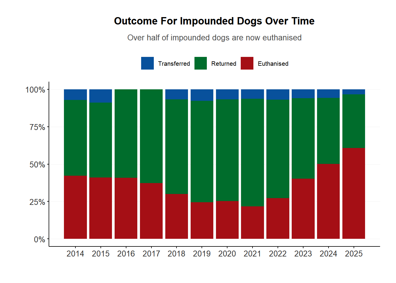
The overall rate of euthanising impounded dogs was dropping between 2014-2019. But after COVID, the rate has increased to be higher than ever before.
<- $ impounds |> filter (category != "impounds" )$ category <- factor (impound_result$ category, levels = c ("transferred" , "returned" , "euthanised" ))ggplot (impound_result, aes (x = year, y = count, fill = category)) + geom_bar (position = "fill" , stat = "identity" ) + scale_fill_manual (values = c ("#08519c" , "#006d2c" , "#a50f15" ),labels = tools:: toTitleCase) + scale_y_continuous (labels = scales:: label_percent ()) + scale_x_continuous (breaks = unique (impound_result$ year)) + xlab ("" ) + ylab ("" ) + plot_theme () + labs (title = "Outcome For Impounded Dogs Over Time" ,subtitle = "Over half of impounded dogs are now euthanised" )
Warning: Removed 2 rows containing missing values or values outside the scale range
(`geom_bar()`).
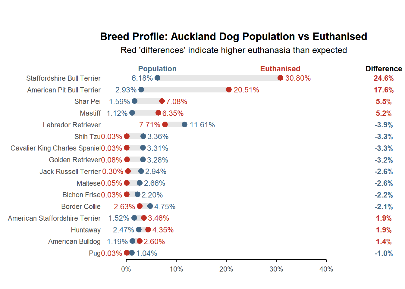
Impound outcome by primary breed (population and impound data are both FY2024)
<- registration |> filter (sheet_name == "FY24" ) |> count (primary_breed = breed_standardised, name = "n_pop" ) |> mutate (prop_pop = n_pop / sum (n_pop)) |> inner_join (|> filter (impound_date > "2023-07-01" , status %in% c ("Euthanised" , "For Euthanasia" )) |> mutate (primary_breed = str_replace (primary_breed, ".*Pit Bull Terrier.*" , "American Pit Bull Terrier" )) |> count (primary_breed, name = "n_euth" ) |> mutate (prop_euth = n_euth / sum (n_euth)),by = "primary_breed" |> mutate (diff = prop_euth - prop_pop,max_val = pmax (prop_euth, prop_pop) |> filter (abs (diff) > 0.01 ) |> arrange (abs (diff)) |> mutate (primary_breed = fct_inorder (primary_breed))<- c ("prop_euth" = "#BF2F24" , "prop_pop" = "#436685" )<- nrow (breed_data)<- breed_data |> pivot_longer (cols = starts_with ("prop" ), names_to = "type" , values_to = "val" ) |> ggplot (aes (val, primary_breed)) + geom_line (aes (group = primary_breed), color = "#E7E7E7" , linewidth = 3.5 ) + geom_point (aes (color = type), size = 3 ) + geom_text (aes (label = percent (val, 0.01 ), color = type, hjust = if_else (val == max_val, - 0.2 , 1.2 )), size = 3.25 ) + geom_text (data = \(.x) filter (.x, primary_breed == last (primary_breed)),aes (label = if_else (type == "prop_pop" , "Population" , "Euthanised" ), color = type),nudge_y = 0.8 , fontface = "bold" , size = 3.25 ) + scale_x_continuous (breaks = seq (0 , 0.4 , by = 0.10 ),labels = \(x) if_else (round (x, 2 ) %in% round (seq (0 , 0.4 , 0.1 ), 2 ), percent (x, accuracy = 1 ), "" ),guide = guide_axis (cap = "both" )+ scale_color_manual (values = colours) + coord_cartesian (xlim = c (- 0.02 , 0.45 ), ylim = c (1 , n_breeds + 1 ), clip = "off" ) + labs (title = "Breed Profile: Auckland Dog Population vs Euthanised" ,subtitle = "Red 'differences' indicate higher euthanasia than expected" , x = NULL , y = NULL ) + theme_minimal () + theme (legend.position = "none" , panel.grid = element_blank (), plot.title = element_text (face = "bold" , hjust = 0.5 ), plot.subtitle = element_text (hjust = 0.5 ),axis.line.x = element_line (color = "black" , linewidth = 0.5 ),axis.ticks.x = element_line (color = "black" , linewidth = 0.5 ),axis.ticks.length.x = unit (3 , "pt" )<- ggplot (breed_data, aes (x = 0 , y = primary_breed)) + geom_text (aes (label = percent (diff, 0.1 ), color = if_else (diff > 0 , "prop_euth" , "prop_pop" )),fontface = "bold" , size = 3.25 ) + annotate ("text" , x = 0 , y = n_breeds + 0.8 , label = "Difference" , fontface = "bold" , size = 3.25 ) + scale_color_manual (values = colours) + coord_cartesian (ylim = c (1 , n_breeds + 1 ), clip = "off" ) + theme_void () + theme (legend.position = "none" )+ p2 + plot_layout (widths = c (10 , 1 )) & theme (plot.margin = margin (20 , 5 , 10 , 5 )) Reasons for euthanasia
<- |> filter (impound_date > "2023-07-01" & ! is.na (euthanasia_reason)) |> mutate (euthanasia_reason = case_when (str_detect (euthanasia_reason, "Health|Parvo" ) ~ "Health or Parvo Virus" ,str_detect (euthanasia_reason, "Dog vs Dog|Dog vs Domestic|Dog vs Stock|Dog vs Poultry" ) ~ "S.57 Dog vs Animal" ,.default = euthanasia_reason|> group_by (euthanasia_reason) |> count (name = "count" ) |> ungroup () |> mutate (proportion = count / sum (count)|> arrange (desc (proportion))
# A tibble: 13 × 3
   euthanasia_reason                 count proportion
   <chr>                             <int>      <dbl>
 1 Failed Temperament Test            1963   0.501
 2 Shelter Full                        948   0.242
 3 Health or Parvo Virus               518   0.132
 4 S.57 Dog vs Animal                  120   0.0306
 5 S.57 Dog vs Person                  106   0.0271
 6 No Longer Suitable For Adoption      86   0.0219
 7 S.57A Aggressive Behaviour           71   0.0181
 8 Dependant Pup                        37   0.00944
 9 Relinquish - Aggressive Behaviour    31   0.00791
10 Destruction Order - S.64             19   0.00485
11 Menacing Dog - S.33A Deed            13   0.00332
12 Dangerous Dog - S.31                  3   0.000766
13 Menacing Dog - S.33C Breed            3   0.000766
Total infringements skyrocket in 2025
$ enforcement |> filter (category == "infringements-total" )
# A tibble: 12 × 3
    year category            count
   <dbl> <chr>               <dbl>
 1  2025 infringements-total 17430
 2  2024 infringements-total  6387
 3  2023 infringements-total  4748
 4  2022 infringements-total  3271
 5  2021 infringements-total  5126
 6  2020 infringements-total  3480
 7  2019 infringements-total  5172
 8  2018 infringements-total  5817
 9  2017 infringements-total  5098
10  2016 infringements-total  3835
11  2015 infringements-total  4521
12  2014 infringements-total  5638
The bulk of infringements are for failing to register a dog
$ enforcement |> filter (category == "failure-register" )
# A tibble: 12 × 3
    year category         count
   <dbl> <chr>            <dbl>
 1  2025 failure-register 10149
 2  2024 failure-register  2305
 3  2023 failure-register  1490
 4  2022 failure-register   763
 5  2021 failure-register  1903
 6  2020 failure-register  1138
 7  2019 failure-register  2028
 8  2018 failure-register  2534
 9  2017 failure-register  2109
10  2016 failure-register  1496
11  2015 failure-register  2200
12  2014 failure-register  3203
But prosecutions remain at low levels
$ enforcement |> filter (category == "prosecutions-appeals" )
# A tibble: 12 × 3
    year category             count
   <dbl> <chr>                <dbl>
 1  2025 prosecutions-appeals   141
 2  2024 prosecutions-appeals   117
 3  2023 prosecutions-appeals   121
 4  2022 prosecutions-appeals   117
 5  2021 prosecutions-appeals   134
 6  2020 prosecutions-appeals   161
 7  2019 prosecutions-appeals   220
 8  2018 prosecutions-appeals   237
 9  2017 prosecutions-appeals   217
10  2016 prosecutions-appeals   197
11  2015 prosecutions-appeals   137
12  2014 prosecutions-appeals   210
Auckland Dog Population By Region
Get Auckland human population by region
# Source: https://figure.nz/chart/bSr6yQmn9V9BFrXK <- read_csv ("../data/2023-auckland-population.csv" ) |> filter (` Census year ` == "2023" & ` Local board area ` != "Auckland" ) |> mutate (local_board = paste0 (` Local board area ` , " Local Board Area" ),local_board = case_when (== "Auckland Local Board Area" ~ "Total Auckland" ,.default = local_board)|> rename (census_year = ` Census year ` ,population = Value) |> select (census_year, local_board, population) |> left_join (locality |> select (local_board, region) |> unique (),by = join_by (local_board)) |> group_by (region) |> reframe (human_population = sum (population)
Rows: 154 Columns: 8
── Column specification ────────────────────────────────────────────────────────
Delimiter: ","
chr (6): Census year, Local board area, Local board area Code, Measure, Valu...
dbl (1): Value
lgl (1): Null Reason

ℹ Use `spec()` to retrieve the full column specification for this data.
ℹ Specify the column types or set `show_col_types = FALSE` to quiet this message.
Known dogs
<- |> filter (sheet_name == "FY25" ) |> left_join (locality, by = join_by (suburb)) |> select (suburb, local_board, region) |> group_by (suburb) |> add_count (suburb, name = "known_suburb" ) |> group_by (local_board) |> add_count (local_board, name = "known_board" ) |> group_by (region) |> add_count (region, name = "known_region" ) |> unique () |> arrange (desc (known_suburb)) |> ungroup ()|> select (region, known_region) |> distinct () |> left_join (auck_pop,by = join_by (region)) |> arrange (desc (known_region)) |> mutate (dogs_per_1k_human = (known_region / human_population) * 1000 ,across (c (known_region, human_population), label_comma ()),region = tools:: toTitleCase (region)|> rename ("Region" = region,"Dogs" = known_region,"People" = human_population,"Dogs Per 1,000 People" = dogs_per_1k_human|> kable () |> kable_styling () Dog population trends in each Local Board
<- |> select (sheet_name, suburb) |> left_join (locality, by = join_by (suburb)) |> group_by (sheet_name, local_board) |> count () |> pivot_wider (names_from = sheet_name, values_from = n) |> mutate (change = (FY25 - FY21) / FY21|> filter (FY25 > 100 ) |> arrange (desc (change)) |> ungroup ()|> mutate (across (contains ("FY" ), comma),change = scales:: percent (change, accuracy = 0.1 )|> rename ("2021" = "FY21" ,"2022" = "FY22" ,"2023" = "FY23" ,"2024" = "FY24" ,"2025" = "FY25" ,"Change" = "change" ,"Local Board" = "local_board" |> kable () |> kable_styling ()
median (dogs_board$ change, na.rm = TRUE ) While the median increase across Auckland local boards was 9%, the Interquartile Range (IQR) analysis below identifies Māngere-Ōtāhuhu and Ōtara-Papatoetoe Local Boards as statistical outliers for their significantly higher growth, distinct from the regional trend.
# Calculate upper fence <- dogs_board |> summarise (q1 = quantile (change, 0.25 ),q3 = quantile (change, 0.75 ),iqr = q3 - q1,upper_fence = q3 + (1.5 * iqr)# Flag high outliers <- dogs_board |> mutate (is_high_outlier = change > stats$ upper_fence,|> filter (is_high_outlier)
# A tibble: 2 × 8
  local_board                FY21  FY22  FY23  FY24  FY25 change is_high_outlier
  <chr>                     <int> <int> <int> <int> <int>  <dbl> <lgl>
1 Māngere-Ōtāhuhu Local Bo…  3407  3677  4173  4670  4809  0.412 TRUE
2 Ōtara-Papatoetoe Local B…  3912  4267  4668  5107  5192  0.327 TRUE
Registration data
<- |> filter (sheet_name == "FY25" ) |> mutate (current_reg = case_when (registration_latest_year < 2024 ~ FALSE , .default = TRUE ),owner_reg = case_when (owner_registration_class == "RDOL" ~ TRUE ),classification = case_when (classification == "Unknown" ~ FALSE ,str_detect (classification, "Menacing|Dangerous" ) ~ TRUE )|> left_join (regions_dogs, by = join_by (suburb)) |> select (current_reg, owner_reg, breed_standardised, animal_desexed, classification, suburb, local_board: known_region) <- |> pivot_longer (cols = c (current_reg, owner_reg, animal_desexed, classification),names_to = "metric" ,values_to = "is_true" |> group_by (suburb, local_board, region, metric) |> summarise (count = sum (is_true, na.rm = TRUE ),known_suburb = first (known_suburb),known_board = first (known_board),known_region = first (known_region),.groups = "drop" |> group_by (metric) |> mutate (p_suburb = count / known_suburb|> group_by (local_board, metric) |> mutate (p_board = sum (count) / first (known_board)) |> group_by (region, metric) |> mutate (p_region = sum (count) / first (known_region)) |> ungroup ()write_csv (regions_reg, "../outputs/regions_reg.csv" ) Compare Local Boards
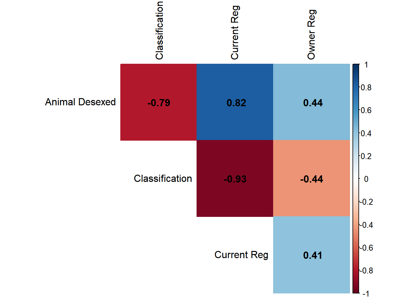
<- regions_reg |> select (local_board, metric, p_board) |> distinct () |> mutate (metric = metric |> str_replace_all ("_" , " " ) |> str_to_title (),local_board = local_board |> str_replace_all ("_" , " " ) |> str_to_title ()<- plot_data |> group_split (metric)<- plots_list |> reduce (\(p_obj, data_slice) {|> add_bars (data = data_slice,x = ~ p_board,y = ~ fct_reorder (local_board, p_board),name = unique (data_slice$ metric),marker = list (color = region_colours[which (plots_list == list (data_slice))]),visible = (identical (data_slice, plots_list[[1 ]])),orientation = 'h' ,showlegend = FALSE ,hovertemplate = "Board: %{y}<br>Value: %{x:.1%}<extra></extra>" .init = plot_ly (height = 800 ))<- plots_list |> imap (\(data_slice, idx) {<- rep (FALSE , length (plots_list))<- TRUE list (method = "restyle" ,args = list ("visible" , as.list (vis_vector)),label = unique (data_slice$ metric)<- p |> layout (title = list (text = "Animal Registration Metrics by Local Board (FY25)" ,x = 0.05 , y = 0.98 , xanchor = 'left' ,yanchor = 'top' ,font = list (size = 20 )margin = list (l = 180 , t = 100 , r = 30 , b = 50 ),xaxis = list (title = "" , tickformat = ".0%" ),yaxis = list (title = "" ),updatemenus = list (list (buttons = buttons,direction = "down" ,showactive = TRUE ,x = 0.10 , y = 1.05 , xanchor = 'left' ,yanchor = 'top' ,bgcolor = "#f8f9fa" :: saveWidget (interactive_plot, "../outputs/reg_metrics.html" , selfcontained = TRUE ) The below Spearman rank correlation analysis shows that Local Boards with high current registrations tend to have high rates of desexing and low rates of classified animals, while those with high rates of classifications tend to have lower rates of desexing.
<- plot_data |> pivot_wider (names_from = metric, values_from = p_board) |> select (- local_board) |> as.matrix ()<- rcorr (corr, type = "spearman" )corrplot (cor_results$ r, method = "color" , type = "upper" , addCoef.col = "black" , tl.col = "black" , diag = FALSE ,sig.level = 0.05 , insig = "blank" ) Attacks per 1,000 known dogs in each Local Board
<- rfs |> filter (>= "2024-07-01" ,str_to_lower (rfs_type) %in% c ("dog attack on people" , "dog attack on child" )|> count (suburb, name = "attacks_suburb" ) |> inner_join (regions_dogs, by = "suburb" ) |> group_by (local_board) |> mutate (attacks_board = sum (attacks_suburb)) |> group_by (region) |> mutate (attacks_region = sum (attacks_suburb)) |> ungroup () |> mutate (rate_suburb = (attacks_suburb / known_suburb) * 1000 ,rate_board = (attacks_board / known_board) * 1000 ,rate_region = (attacks_region / known_region) * 1000 |> select (suburb, local_board, region, starts_with ("attacks" ), starts_with ("known" ), starts_with ("rate" ))write_csv (regions_attacks, "../outputs/regions_attacks.csv" ) Primary breed profile for each region
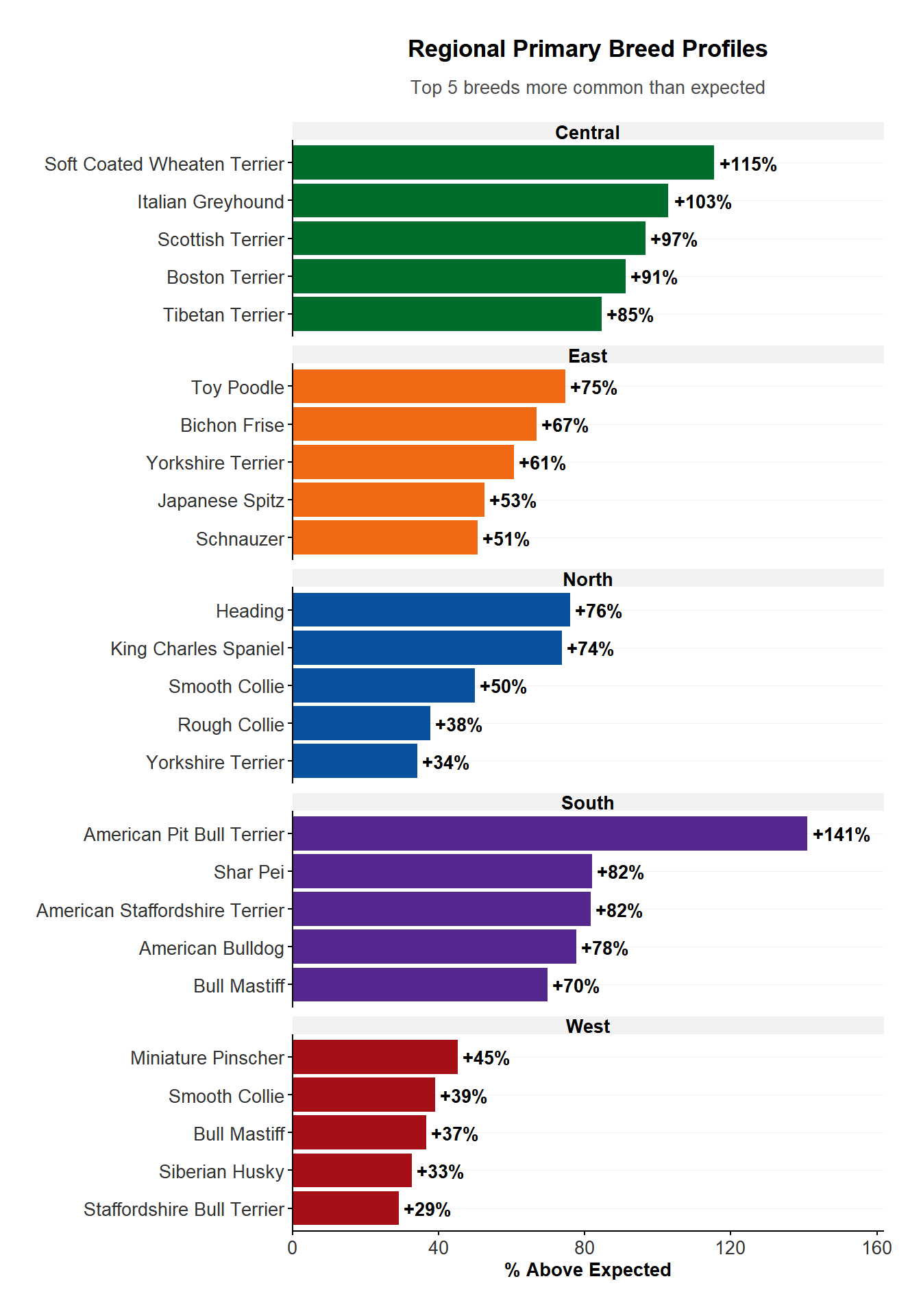
<- |> filter (sheet_name == "FY25" ) |> left_join (locality, by = join_by (suburb)) |> group_by (region) |> count (breed_standardised, name = "count" ) |> arrange (desc (count), .by_group = TRUE ) |> left_join (regions_dogs |> select (region, known_region) |> unique (), by = join_by (region)) |> mutate (prop_breed = format (count / known_region, scientific = FALSE ) Compare regional breed profiles statistically
<- regions_breed |> perform_chisq (group_var = "region" , cat_var = "breed_standardised" , count_var = "count"
Warning: Use of .data in tidyselect expressions was deprecated in tidyselect 1.2.0.
ℹ Please use `all_of(var)` (or `any_of(var)`) instead of `.data[[var]]`
write_csv (breeds_region, "../outputs/breed_over.csv" )
|> group_by (group) |> slice_max (percent_diff, n = 5 ) |> ungroup () |> ggplot (aes (x = reorder_within (category, percent_diff, group), y = percent_diff, fill = group)) + geom_col () + scale_fill_manual (values = region_colours) + geom_text (aes (label = paste0 ("+" , round (percent_diff), "%" )), hjust = - 0.1 , size = 3.5 , fontface = "bold" ) + scale_x_reordered () + coord_flip () + facet_wrap (~ group, scales = "free_y" , ncol = 1 ,labeller = function (labels) {lapply (labels, tools:: toTitleCase)+ scale_y_continuous (expand = expansion (mult = c (0 , 0.15 ))) + plot_theme () + theme (legend.position = "none" ) + labs (title = "Regional Primary Breed Profiles" ,subtitle = "Top 5 breeds more common than expected" ,x = NULL , y = "% Above Expected" Impounds per 1,000 dogs (FY2024 data)
<- impounds |> filter (impound_date > "2023-07-01" ) |> count (suburb, name = "impounds_suburb" ) |> inner_join (locality, by = "suburb" ) |> left_join (regions_dogs |> select (local_board, known_board, known_region), by = "local_board" ) |> unique () |> group_by (local_board) |> mutate (impounds_board = sum (impounds_suburb)) |> group_by (region) |> mutate (impounds_region = sum (impounds_suburb)) |> ungroup () |> mutate (rate_board = (impounds_board / known_board) * 1000 ,rate_region = (impounds_region / known_region) * 1000 |> select (suburb, local_board, region, starts_with ("impounds" ), starts_with ("known" ), starts_with ("rate" ))
Warning in left_join(inner_join(count(filter(impounds, impound_date > "2023-07-01"), : Detected an unexpected many-to-many relationship between `x` and `y`.
ℹ Row 1 of `x` matches multiple rows in `y`.
ℹ Row 23 of `y` matches multiple rows in `x`.
ℹ If a many-to-many relationship is expected, set `relationship =
  "many-to-many"` to silence this warning.
write_csv (regions_impounds, "../outputs/regions_impounds.csv" ) Impound rate for attacks/rushing (FY2024 data)
<- c ("Relq - Sec 57" , "Sec 57" )<- c ("Sec 57A" )<- impounds |> filter (> "2023-07-01" ,%in% c (attack_codes, rush_codes)|> count (suburb, name = "impounds_attack_suburb" ) |> inner_join (locality, by = "suburb" ) |> left_join (regions_dogs |> select (local_board, known_board, known_region), by = "local_board" ) |> unique () |> group_by (local_board) |> mutate (impounds_attack_board = sum (impounds_attack_suburb, na.rm = TRUE )) |> group_by (region) |> mutate (impounds_attack_region = sum (impounds_attack_suburb, na.rm = TRUE )) |> ungroup () |> mutate (across (starts_with ("known" ), ~ replace_na (.x, 0 )),rate_attack_board = (impounds_attack_board / known_board) * 1000 ,rate_attack_region = (impounds_attack_region / known_region) * 1000 |> mutate (across (starts_with ("rate" ), ~ if_else (is.infinite (.x), NA_real_ , .x))) |> select (suburb, local_board, region, starts_with ("impounds" ), starts_with ("known" ), starts_with ("rate_attack" ))
Warning in left_join(inner_join(count(filter(impounds, impound_date > "2023-07-01", : Detected an unexpected many-to-many relationship between `x` and `y`.
ℹ Row 1 of `x` matches multiple rows in `y`.
ℹ Row 29 of `y` matches multiple rows in `x`.
ℹ If a many-to-many relationship is expected, set `relationship =
  "many-to-many"` to silence this warning.
write_csv (regions_impounds_attacks, "../outputs/regions_impounds_attacks.csv" ) Outcome of impound by area
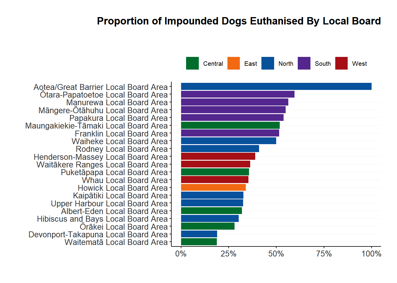
<- impounds |> filter (impound_date > "2023-07-01" ) |> mutate (status = case_match (status, "For Euthanasia" ~ "Euthanised" ,c ("Adoption Pending" , "Fostered" , "Hold - Adoption" ) ~ "Adopted" ,c ("Trfd to Breed Rescue" , "Trfd to Other TA" , "Trfd to Rescue Group" , "Trfd to SPCA" ) ~ "Rescued" ,c ("Dead on Arrival" , "Died in Shelter" , "Escaped" , "Hold - General" , "Hold - Legal Reason" , "Hold - Temp Test" , "Processing" , "Stolen" ) ~ "Other" ,.default = status|> left_join (regions_dogs, by = "suburb" ) |> count (region, local_board, status, name = "count" ) |> group_by (local_board) |> mutate (board_total = sum (count),proportion = count / board_total|> ungroup ()
Warning: There was 1 warning in `mutate()`.
ℹ In argument: `status = case_match(...)`.
Caused by warning:
! `case_match()` was deprecated in dplyr 1.2.0.
ℹ Please use `recode_values()` instead.
write_csv (regions_impounds_outcome, "../outputs/regions_impounds_outcome.csv" )|> filter (status == "Euthanised" & ! is.na (local_board)) |> ggplot (aes (x = fct_reorder (local_board, proportion), y = proportion, fill = region)) + geom_col () + coord_flip () + scale_fill_manual (values = region_colours,labels = stringr:: str_to_title) + scale_y_continuous (labels = scales:: label_percent ()) + plot_theme () + theme (plot.title = element_text (hjust = 1 )) + labs (title = "Proportion of Impounded Dogs Euthanised By Local Board" ,subtitle = "" ) + xlab ("" ) + ylab ("" ) Impounds by breed
<- impounds |> filter (impound_date > "2023-07-01" ) |> count (primary_breed, name = "impound_count" ) |> inner_join (|> select (- prop),by = join_by (primary_breed == breed_standardised)|> mutate (impound_rate = round ((impound_count / primary_breed.y) * 1000 , digits = 1 )) |> filter (primary_breed.y > 99 ) |> arrange (desc (impound_rate)) |> head (n = 10 )|> rename ("Breed" = primary_breed,"Impounds" = impound_count,"Population" = primary_breed.y,"Impound Rate" = impound_rate) |> mutate (across (c (` Impounds ` , ` Population ` ), ~ format (.,big.mark = "," ))|> kable () |> kable_styling ()